Function Interpolation and Approximation

Let say that the temperature at the noon is 14⁰C and two hours later it increase to 16⁰C. What is the temperature at 1 pm.? Of course, we can't know exactly what was the temperature at 1p.m. based on these two values but we are rather sure that it was somewhat between.

In many situation, in science and engineering and other areas we need a concrete figure as the answer to the question like above one. Among many possible ways of the temperature change from noon to 2 pm., we can assume the one for which the temperature at 1 pm. was 15⁰C. This is easy to calculate (the value is the mean of the two values since 1 pm is in the middle of the given period) and the most probably close to the real value.

The method we just describe on this simple example is called linear interpolation. Among the interpolation methods linear interpolation is conceptually the simplest and it is often used.

Two basic method of function interpolation are interpolations by

• Lagrange polynomial and
• Newton polynomial.

In this article we will describe, explain and illustrate both of techniques. One can find a concrete case study that compare the two procedure on the same data (see Example 1 and Example 2).

In many occasions we don't know analytical expression of some function f but only its values in several points: x₀<x₁<x₂<...<x_n. Situations like these demand to calculate i.e. to estimate the function value in some points different than the given ones – for which we know the value of function. A procedure of determination of function g on the interval [x₀,x_n] where it holds

g(x_i)=f(x_i), i=0,1,2,...

is called function interpolation.

A function g can be chose from the class of polynomials, trigonometric, rational and other function. Probable the most common is polynomial interpolation (i.e. linear and polynomial since a polynomial of the degree two we call linear function).

Close to the term function interpolation is approximation of a function. The main difference is that within interpolation we are looking for "a missing value" between the two known function values while within approximation we are looking for a simpler function replacing a complex one (which is either known or unknown). While obtained function within interpolation have to contain all already known values it is not case in approximation. In that case obtain function have to fit known values "as best as possible" – the criterion for this adhesion is usually defined by the minimum squares method. Function approximation will be explained later in this article.

Now, polynomial interpolation will be exposed by means of two methods i.e. using the Lagrange polynomial and Newton polynomial.

Let the pair of points (x₀,f(x₀)), (x₁,f(x₁)),...,(x_n,f(x_n)) are given, representing known values of a function. The general expression of Lagrange polynomial then is

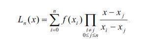
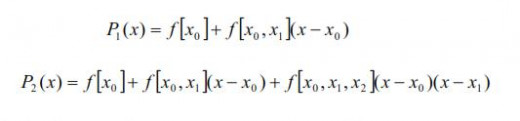
For Lagrange polynomials of the degrees one and two it holds:

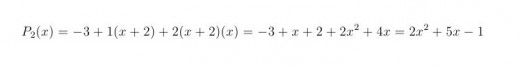
Example 1. What is the Lagrange polynomial which graph contains the points T₀(-2,-3), T₁(0,-1) and T₂(1,6).

Since we have three function value known, polynomial of the degree two will be chosen. Lagrange polynomial of the degree two is presented on the figure above. Substituting the values we get:

Thus, the solution is polynomial 2x²+5x-1 which graph is presented on the first figure. It is visible that the graph contain all three given points.

The general expression of Newton polynomial is given by

where

As an illustration, it follows Newton polynomials of the degrees one and two.

Calculation of the coefficients in Newton polynomial is practical if one use this differences table:

Contrary to Lagrange method, here one can additionally add a new pair of points (adding one sequence in the table). Furthermore, if some of data changes it is not necessary to count all over again but only the related differences.

The next example illustrates the method on the same case as we have in the first example.

Example 2. For the points T₀(-2,-3), T₁(0,-1) and T₂(1,6) find interpolation polynomial by means of Newton's method.

Firstly, the table of differences should be determined:

As a second and final step, coefficients obtained by the table above we substitute in the Newton polynomial of the degree two. As we expected, the solution is the same as in case when Lagrange method were used.

In the above we dealt with function interpolation, which means that that function f is replaced by a function g so that its value are equal in the given points.

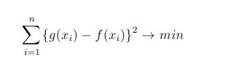
Here we should to replace a function f with some more simple function that will “very well present f on the whole domain. The “quality” of the approximation will be measured by minimum sum squares method. More precisely, a function g have to be determined, with the following condition, where n is the number of known function value:

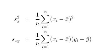
Let pairs (x₁,y₁), (x₂,y₂),...,(x_n,y_n) represent n known values of the function f. The equations of linear function which approximate the given set my means of minimum sum squares method is

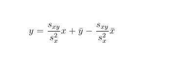
where we have the mean of both x and y values and where it holds

Example 3. Given the set of points as in the table below, we have to find linear function by means of minimum squares method.

The whole calculation can be seen in the next table. Once we substitute the obtained values (the last row in the table) in the general linear function equation above, final solution follows: g(x)=0.951192*x+0.092724.

The obtained function g and previously given data one can see in the next figure.

A video at the end shows how we can use function interpolation in order to find a missing data. In this example we use the simplest possible case- linear interpolation. Although linear interpolation is the simplest type of interpolation it is suitable in most of the situations.