Mild and Wild Randomness (normal distribution vs Cauchy distribution)

The first association on the term “randomness” is usually casino, toss of a coin, toss of a dice... One may think on casino as a place of huge uncertainty. However, this uncertainty is much more predictable and much less haphazard than some another random processes. Not all randomness are (qualitatively) equal!

In this article two types of randomness will be discussed through its representatives. For mild randomness we have bell shape distribution, called Gaussian distribution. On the opposite side, for wild randomness we have Cauchy distribution. In the fist case, there is negligible probability for extreme events whereas in the second case we have have so called “fat tail”. Although we can't know what will be the score of the next roulette game, neither we know the result of the next toss of a dice, in such a cases we have a macroscopic certainty.

What would be the number of score "6" after 600 toss of a dice? As we know, according to the definition, probability is the ratio of the number of desired outcomes and the number of possible events. Due to this fact we expect around 100 scores "6". What is our expectation if we toss a dice 6000 times? Again, we expect 1/6 of throws; and according to the low of large numbers, in this case, the number of desired outcomes will be closer (in percentage) to the figure of 1000 than in previous case to the figure of 100. So, the larger number of throws the smaller deviation from the expected value.

Let imagine a blindfolded archers trying to hit a target on a wall. For each snapshot, we measure the distance from the center of the target. What average distance one can expect after 100, 1000, 1000 shots? Is there any expected value? - in this case there is no any expected value. As the archer continue with snap shots, the average distance will change its value without tendency to any value. Namely, such a random process is essentially different than the process of toss of a coin. This is an example of a process where random variable has no expected value – as it is case with toss of a coin.

The first case is an example of so called mild randomness, meaning that there is a macroscopic certainty. We can't know the result of any particular experiment but we know the result of a large series of experiments. There is no possibility that one particular test significantly influence the majority of tests. However, in the second case there is no any certainty. There is always a possibility that the result of the next test radically influence the average of previous tests.

A distribution without the law of large numbers

In the experiment with a rotating line (see figure below), the random variable is the distance x. However, performing several series of measures, one can see that the average of x does not aspire to some constant value, i.e. the law of large numbers doesn't hold here.

In the 19 th century one of a field of interest for mathematicians was calculation of orbital elements of celestial bodies (astronomy was a branch of mathematics in that time). It was known that telescopes are not absolutely precise but there is some systematic error in observation. This problem occupied both Gauss and Lagendre, and they developed (independently) a theoretical distribution that is nowadays called Gaussian distribution or normal distribution. Lagendre was first with his work (1805) while Gauss explain the theory better (1809).

It can be said that Gaussian distribution is widespread: it appears in several cases in mathematics, it has many nice mathematical properties (symmetry being the obvious one), it appears in quantum mechanics as well. However, there is no many random variables with normal distribution. In related books one can usually find the two examples: toss of a coin and toss of a dice. While it is possible to find normally distributed random variable in physics, it seems that such a distribution is not typical for socio-economical phenomena. For example, the speed of gas molecules is distributed as a Gaussian random variable. In his very popular book “The Black Swan”, N. Taleb said that randomness of Gaussian type are not present in socio-economical phenomena.

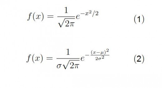
The Gaussian distribution (or normal distribution) is a continuous probability distribution, defined by the probability density function (1) for standard case and (2) in general. Standard case means the average of 0 and standard deviation of 1. Notation of this distribution is N(μσ²).

The function is symmetric, having maximal value when x is the mean. The expected value of this distribution is the mean. Mean, median and mode for this distribution are all equal to each other. The inflection points of the curve are one standard deviation away from the mean, at points x=μ-σ, and x=μ+σ. It is known that with probability 95% a random variable distributed on this way will take a value within two standard deviation away from the mean. With probability of 99.7%, a random variable will takes the value in the interval of three standard deviation from the mean. Thus, after 3σ probability is negligible. This fact is known as "68-95-99 rule" or 3-sigma rule. (There is 68% probability that a random variable will takes the value within 1 sigma away from the mean.) Informally, this distribution is also called the bell curve.

This distribution appears theoretically in several parts of mathematics, including probability theory and Fourier analysis. It appears theoretically in quantum mechanics as well. In physics, velocity of molecules of gas is normally distributed. Based on this distribution, Albert Einstein explain the random motion of grains of pollen of the plant- which was firstly observed by Scottish botanist Robert Brown. The most known examples of a random processes that behave this way are toss of a coin and toss of a dice.

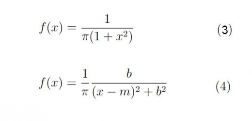
In probability theory, the Cauchy distribution is a continuous probability distribution, defined by the probability density function (3) for standard case and (4) in general. This function is symmetric as well, having maximum at the median. The mean is not defined for this distribution while the mode is equal to the median.

Contrary to the Gaussian distribution within Cauchy distribution there is no expected value. Expected value for this distribution is not defined (since the definite integral defining expected value has no finite value). This means that in this case the low of large numbers doesn't hold. Because of this sensitivity on extreme events this distribution, as well as the others with the same property, is called the distribution with fat tail. This distribution is also known as Lorentz distribution of Cauchy-Lorentz distribution.

One remarkable application of this distribution is in physics, where it describes amplitude in a resonance effect. Another one example of such a distribution is rotation of a line around a point (see figure), where the distance x is the random variable. If the angle is randomly chosen, then random variable x has the Cauchy distribution. The next table shows results of experiments showing there is no expected value. In the first column we see the number of series of tests whereas in every series we have 10 experiments. Obviously, there the low of large numbers doesn't hold in this case.

Besides, parameters of financial markets are examples of distribution with "fat tail" i.e. distribution with significan probability for extreme events.

The basic parameter on the financial markets is the price change. Usually we deal with a daily price change, that is expressed in percentage. Thus, the price change is a random variable, in a terminology of probability theory. The question is how this variable is distributed? Is it a kind of mild probability or wild?

It seems that price changes behave very unpredictable i.e. wild in this means. As we know, markets are very risk places with reported very extreme occurrences. Few times there were so huge changes on the market that that day are given names in a financial world. This is the case for October 19, 1987 that is called the black Monday. On this day markets throughout the world, from America and Europe to Asia, drooped for in most cased for 40%. New Zeland stock exchange reported even worse loss.

During the crisis in 1929 one of the worst day on markets was September 18, called the black Thursday.

Thus, mild randomness is every random process which can be described by normally distributed random variable. On the opposite side there is so called wild randomness, representing random processes with significant probability of extreme events. In case of Gaussian distribution, there is only 0.3% probability that random variable takes a value more than 3 standard deviation apart from the mean.

So, extreme event has probability which is in probability theory called practically impossible event. An example of wild randomness is Cauchy distribution, a distribution without defined the expected value and with property that events very far away from the median are possible.

In the prologue of his book "The misbehavior of markets", Benoit Mandelbrot says:

"Three states of matter – solid, liquid and gas – have long been known. An analogous distinction between three states of randomness – mild, slow and wild – arises from the mathematics of fractal geometry."

So, in addition to mild and wild randomness we deal with in this article, there is also something between, called "show" randomness. Actually, there is the whole class of distribution between Gaussian and Cauchy distribution, called L-stable distribution. More precisely, Gaussian and Cauchy distribution are on the marginal sides of these class.